Ordered	Unordered	Ordered-Unordered
Correlation	Spearman's rho	Cramer's V	Cramer's V
Question Order Bias	Mann-Whitney U-Test	Chi-Squared Test	N/A
Question Wording Bias	Mann-Whitney U-Test	Chi-Squared Test	N/A
Breakoff	Nonparametric Bootstrap	Nonparametric Bootstrap	N/A
Bad Actors	Nonparametric Bootstrap on Empirical Entropy	Nonparametric Bootstrap on Empirical Entropy	N/A

Correlation

Recall that correlation is typically measured as the degree to which two variables covary. We are generally interested in correlation as a measure of predictive power. Correlation coefficients give the magnitude of a monotone relationship between two variables. Completely random responses for two questions will result in a low correlation coefficient.

We use two measures of correlation. For ordered questions, we use Spearman’s $$\rho$$; this coefficient ranks responses and measures to degree to which the ranked results have a monotone relationship. For unordered questions, we use Cramer’s $$V$$. The procedure for Cramer’s $$V$$ is based on the $$\chi^2$$ statistic; we take one question and compute the empirical probability for each answer. We then use this estimator to compute the expected values for each of the values in the other question and find the normalized differences between observed and expected values. The sum of these values is the $$\chi^2$$ statistic, which has a known distribution. Cramer’s $$V$$ scales the value of the $$\chi^2$$ statistic by the sample size and the minimum degrees of freedom.

Both of these tests are sensitive to small counts for some categories. We generally do not collect sufficient information to produce meaningful confidence intervals; as a result, we simply flag correlations that may be of interest.

Order Bias

We use the $$\chi^2$$ statistic directly to compute order bias for unordered questions. For any question pair $$q_i, q_j, i\neq j$$, we partition the sample into two sets : $$S_{i<j}$$, the set of questions where $$q_i$$ precedes $$q_j$$ and $$S_{j<i}$$, the set of questions where $$q_i$$ follows $$q_j$$. We assume each set is independent.* We show wolog how to test for bias in $$q_i$$ when $$q_j$$ precedes it:

1. Compute frequencies $$f_{i<j}$$ for the answer options of $$q_i$$ in the set of responses $$S_{i<j}$$. We will use these values to compute the estimator.
2. Compute frequencies $$f_{j<i}$$ for answer options $$q_i$$ in the set of responses $$S_{j<i}$$. These will be our observations.
3. Compute the $$\chi^2$$ statistic on the data set. The degrees of freedom will be one less than the number of answer options, squared. If the probability of computing such a number is less than the value at the $$\chi^2$$ distribution with these parameters, there is a significant difference in the ordering

We compute these values for every unique question pair.

Wording

Wording bias classified in the same was as order bias, except in this case, instead of comparing two sets of responses, we compare $$k$$ sets of responses, corresponding to the number of variants we are interested in.

Breakoff

We address two kinds of breakoff : ones determined by position, and ones determined by question. For both analyses, we use the nonparametric bootstrap procedure to determine a one-sided 95% confidence intervals and flag indices and questions whose counts exceed the threshhold.

Breakoff by position is often an indicator that the survey is too long. Breakoff by question may indicate that a question is unclear, offensive, or burdensome to the respondent. There are also some cases where breakoff may indicate a kind of order bias.

Adversaries

We’ve tried a variety of methods for detecting adversaries. The bests empirical results we’ve seen so far have been for a method that uses entropy.

We first compute the empirical probabilities for each question’s answer options. Then for every response $$r$$, we calculate a score styled after entropy : $$score_{r} = \sum_{i=1}^n p(o_{r,q_i}) * \log_2(p(o_{r,q_i}))$$. We then use the bootstrap method to find a one-sided 95% confidence interval and flag any responses that are above the threshold.

*Independence is based on the assumption that each worker is truly unique and that workers do not collude.

We ran a survey previously conducted by Brian Smith four times, to test our techniques against a gold-standard data set.

Date launched	Time of Day launched (EST)	Total Responses	Unique Respondents	Breakoff?
Tue Sep 17 2013	Morning 9:53:35 AM EST	43	38	No
Fri Nov 15 2013	Night	90	67	Yes
Fri Jan 10 2013	Morning	148	129	Yes
Thu Mar 13 2014	Night 11:49:18 PM EST	157	157	Yes

This survey consists of three blocks. The first block asks demographic questions : age and whether the respondent is a native speaker of English. The second block contains 96 Likert-scale questions. The final block consists of one freetext question, asking the respondent to provide any feedback they might have about the survey.

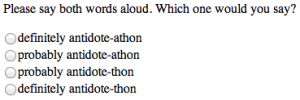
Each of the 96 questions in the second block asks the respondent to read aloud an English word suffixed with either of the pairs “-thon/-athon” or “licious/-alicious” and judge which sounds more like an English word.

First Run

The first time we ran the survey was early in SurveyMan’s development. We had not yet devised a way to measure breakoff and had no quality control mechanisms. Question and option position were not returned We sent the data we collected to Joe Pater and Brian Smith. Brian reported back :

The results don’t look amazing, but this is also not much data compared to the last experiment. This one contains six items for each group, and only 26 speakers (cf. to 107 speakers and 10 items for each group in the Language paper).

Also, these distributions are *much* closer to 50-50 than the older results were. The fact that -athon is only getting 60% in the final-stress context is kind of shocking, given that it gets 90% schwa in my last experiment and the corpus data. Some good news though — the finding that schwa is more likely in -(a)thon than -(a)licious is repeated in the MTurk data.

Recall that the predictions of the Language-wide Constraints Hypothesis are that:
1. final stress (Final) should be greater than non-final stress (noFinal), for all contexts. This prediction looks like it obtains here.
2. noRR should be greater than RR for -(a)licious, but not -(a)thon. Less great here. We find an effect for -thon, and a weaker effect for -licious.

licious (proportion schwaful)

noRR RR
Final 0.5276074 0.5182927
noFinal 0.4887218 0.5031056

thon (proportion schwaful)

noRR RR
Final 0.5950920 0.5670732
noFinal 0.5522388 0.4938272

Our colleagues felt that this made a strong case for automating some quality control.

Second Run

The second time we ran this experiment, we permitted breakoff and used a Mechanical Turk qualification to screen respondents. We required that respondents have completed at least one HIT and have an approval rate of at least 80% (this is actually quite a low approval rate by AMT standards). We asked respondents to refrain from accepting this HIT twice, but did not reject their work if they did so. Although we could have used qualifications to screen respondents on the basis of country, we instead permitted non-native speakers to answer, and then screened them from our analysis. In future versions, we would recommend making the native speaker question a branch question instead.

We performed three types of analyses on this second run of the survey : we filtered suspected bots, we flagged breakoff questions and positions, and we did correlation analysis.

Of the 67 unique respondents in this second run of the phonology survey, we had 46 self-reported native English speakers. We flagged 3 respondents as bad actors. Since we do not have full randomization for Likert scale questions, we use positional preference to flag potential adversaries. Since symmetric positions are equally likely to hold one extreme or another, we say that we expect the number of responses in either of the symmetric positions to be equal. If there is a disproportionate number of responses in a particular position, we consider this bad behavior and will flag it. Note that this method does not address random respondents.

Our three flagged respondents had the following positional frequencies (compared with the expected number, used as our classification threshold). The total answered are out of the 96 questions that comprise the core of the study.

Position 1	Position 2	Position 3	Position 4	Total Answered
82 >= 57.829081	4	10	0	96
0	84 >= 64.422350	9	3	96
28 >= 24.508119	10	0	1	39

We calculated statistically significant breakoff for both question and position at counts above 1. We use the bootstrap to calculate confidence intervals and round the counts up to the nearest whole number. Due to the small sample size in comparison with the survey length, these particular results should be viewed cautiously:

Position	Count
40	2
44	2
49	3
66	2
97	20

Wording Instance (Question)	Suffix	Count
‘marine’	‘thon’	2
‘china’	‘thon’	2
‘drama’	‘thon’	2
‘estate’	‘thon’	2
‘antidote’	‘thon’	4
‘office’	‘licious’	2
‘eleven’	‘thon’	2
‘affidavit’	‘licious’	2

Two features jump out at us for the positional breakoff table. We clearly have significant breakoff at question 98 (index 97). Recall that we have 96 questions in the central block, two questions in the first block, and one question in the last block. Clearly a large number of people are submitting responses without feedback. The other feature we’d like to note is how there is some clustering in the 40s – this might indicate that there is a subpopulation who does not want to risk nonpayment due to our pricing scheme and has determined that breakoff is optimal at this point. Since we do not advertise the number of questions or the amount we will pay for bonuses, respondents must decide whether the risk of not knowing the level of compensation is worth continuing.

Like Cramer’s $$V$$, we flag cases where Spearman’s $$\rho$$ are greater than 0.5. We do not typically have sufficient data to perform hypothesis testing on whether or not there is a correlation, so we flag all found strong correlations.

The correlation results from this run of the survey were not good. We had 6 schwa-final words and 6 vowel-final words. There are 15 unique comparisons for each set. Only 5 pairs of schwa-final words and 3 pairs of vowel-final were found to be correlated in the -thon responses. 9 pairs of schwa-final words and 1 pair of vowel-final words were found to be correlated in the -licious responses. If we raised the correlation threshold to 0.7, none of the schwa-final pairs were flagged and only 1 of the vowel-final pairs was flagged in each case. Seven additional pairs were flagged as correlated for -thon and 3 additional pairs were flagged for -licious.

Third Run

The third run of the survey used no qualifications. We had hoped to attract bots with this run of the survey. Recall that in the previous survey we filtered respondents using AMT Qualifications. Our hypothesis was that bots would submit results immediately.

This run of the survey was the first in this series to be launched during the work day (EST). We obtained 148 total responses, of which 129 were unique. 113 unique respondents claimed to be native English speakers. Of these, we classified 8 as bad actors.

Position 1	Position 2	Position 3	Position 4	Total Answered
23 >= 21.104563	41	31	1	96
0	3	51 >= 40.656844	38 >= 30.456324	92
25 >= 22.476329	39	31	1	96
	29	67 >= 66.209126		96
6	12	43 >= 41.282716	21	82
0	4	42 >= 35.604696	50 >= 38.141304	96
6	28	32	30 >= 29.150767	96
25	0	3	68 >= 64.422350	96

Clearly there are some responses that are just barely past the threshold for adversary detection ; the classification scheme we use is conservative.

Interestingly, we did not get the behavior we were courting for breakoff. Only the penultimate index had statistically significant breakoff; 51 respondents did not provide written feedback. We found 9 words with statistically significant breakoff at abandonment counts greater than 2 (they all had counts of 3 or 4). The only words to overlap with the previous run were “estate” and “antidote”. The endings for both words differed between runs.

As in the previous run, only 5 pairs of schwa-final words plus -thon had correlations above 0.5. Fewer vowel-final pairs (2, as opposed to 3) plus -thon were considered correlated. For the -licious suffix, 10 out of 15 pairs of schwa-final words had significant correlation, compared with 9 out of 15 in the previous run. As in the previous run, only 1 pair of vowel-final words plus -licious had a correlation coefficient above 0.5. This results do not differ considerably from the previous run.

Fourth Run

This run was executed close to midnight EST on a Friday. Of the 157 respondents, 98 reported being native English speakers. We found 83 responses that were not classified as adversaries. Below are the 15 bad actors’ responses:

Position 1	Position 2	Position 3	Position 4	Total Answered
65 >= 64.422350	3	0	28	96
29 >= 25.847473	2	0	2	33
0	5	87 >= 63.825733	4	96
9	18	19	37 >= 35.604696	83
13	2	18	52 >= 47.483392	85
53 >= 40.029801	2	1	0	56
96 >= 66.209126			0	96
3	12	40 >= 39.401554	41 >= 34.327636	96
1	3	5	17 >= 16.884783	26
3	1	1	91 >= 65.018449	96
36 >= 33.044204	42 >= 40.656844	12	6	96
6	32 >= 29.804578	5	0	43
35 >= 30.456324	41	17	3	96
20 >= 19.716955	18	11	2	51
0	0	5	91 >= 63.228589	96

For the -thon pairs, 1 out of the 15 schwa correlations was correctly detected. None of the vowel correlations correctly were detected. For -licious, 2 schwa pair correlations were correctly detected and 4 vowel pair correlations where correctly detected.

For this survey we calculated statistically significant breakoff for individual questions when their counts were above 2 and for positions when their counts were above 1. The penultimate question had 38 instances of breakoff. Fourteen questions had breakoff. The maximum cases were 4 counts each for “cayenne” and “hero” for the suffix -licious.

Entropy Comparison

We observed the following entropies over the 96 questions of interest. Note that the maximum entropy for this section of the survey is 192.

Instance	Initial Entropy	Entropy after removing adversaries
Fourth Run	186.51791933021704	183.64368029571745
Third Run	173.14288208850118	169.58411284759356
Second Run	172.68764654915321	169.15343722609836

Notes

Due to a bug in the initial analysis in the last survey (we changed formats between the third and the fourth), the first run of the analysis did not filter out any non-native English speakers and ran the analysis on 137 respondents. There were 20 adversaries calculated in total and only a handful of correlations detected. The entropy before filtering was 190.0 and after, 188.0. We also counted higher thresholds for breakoff. We believe this illustrates the impact of a few bad actors on the whole analysis.

Note that we compute breakoff using the last question answered. A respondent cannot submit results without selecting some option; without doing this, the “Submit Early” button generally will not appear. However, for the first three runs of the survey, we supplied custom Javascript to allow users to submit without writing in the the text box for the last question.

We need some way of determining whether the diagnoses of SurveyMan’s bugs is correct. It’s always possible that a particular technique has a flaw in it, or that a test for a certain feature is not sensitive enough to detect the differences we would like it to detect. We have designed a simulator as a sanity check for our algorithms.

Simulator setup

The first step in our simulator setup is to generate gold-standard data; this is after all the reason for bothering with a simulator in the first place.

Consider the problem of bot detection. We will need to know the ground truth of who is a bot and who is not. Modeling bots explicitly is easy. We already do this in our static analysis. Modeling human respondents is more challenging.

We define a profile to be a collection of preferences over a survey. These preferences are the probabilities that an instance of a profile (i.e. a respondent) will choose a particular answer option for a question. For example, uniform adversaries will choose each answer option with equal probability.

In order to emulate human behavior, we allow the non-bot population of responses to be drawn from some number of clusters. A cluster is generated by randomly assigning a probabilities $$p_1$$ drawn from the interval $$(1/m_i, 1)$$ for each $$q_i$$. We say that a respondent belonging to one of these clusters has a preference for a particular answer, but may choose another answer due to factors we either cannot control or did not account for. These other preferences are assigned uniform probability : $$\frac{1-p_i}{m-1}$$. Sometimes a preference will be very strong (e.g. assigned a probability > 0.8). Sometimes the preference will only be slight, in which case it will be close to $$1/m_i$$.

We can then inject biases into the generated responses and test our bias detection algorithms, testing the robustness of our techniques by varying the impact of bad actors on our results.

Correlation

Any measure of correlation between questions in the survey must consider what’s called the “level of measurement” of each question. Levels of measurement determine the statistical tools we can use to analyze the data. There are four levels of measurement in total:

1. Nominal Data that fall into categories that have no order are said to be nominal. Generally this will correspond to radio button questions such as “What is your gender.” This data will be represented by a categorical variable and permutation tests will have to be used to analyze any correlations. Tests on nominal data are sensitive to sparsity; since they are not continuous, we cannot use interpolation to make inferences.
2. Ordinal Ordered questions fall into this category. This is probably the most common type of survey question. Surveys that ask users about their preferences or to provide rankings for data are using ordinal data. The more common and powerful statistical significance and correlation tests begin at this level.
3. Interval Where ordinal questions required the ability to rank, interval questions require there to be meaningful distances between answer options. Likert scale questions are an attempt to capture interval questions (although they are often analyzed using ordinal tests, since their measurement is imperfect). Interval questions attempt to capture the magnitude of difference between ranked answers.
4. Ratio Ratio questions are “true” numeric questions – that is, individual answers have meaningful magnitude because there is a known underlying zero grounding the measurement. Weight, date of birth, and income are all ratio questions. These questions permit the most powerful statistical tests because data can be interpolated.

SurveyMan uses correlation in two ways. The CORRELATED can be used to flag sets of questions that the survey designer expects to have statistical correlation. Flagged questions can be used to validate or reject hypotheses and to help detect bad actors. Alternatively, if a question that is not marked as correlated is found to have statistically significant correlation, then we flag this question. Questions are compared on a pair-wise basis. This information can be used in a variety of ways :

• The survey designer could decide to remove one or more of the correlated questions, if their predictive power is strong enough to infer responses from the remaining questions. It is ultimately the responsibility of the survey designer to use good judgement and domain knowledge when deciding to remove questions; note that because we only check pair-wise correlation, we cannot capture the impact of groups on a particular outcome. We do not model interactions between variables.
• The survey designer could use discovered correlations to assist in identification of cohorts or bad actors by updating the entries in the CORRELATED column appropriately.

We only support automated correlation analysis between exclusive (radio button) questions. These questions may be ordered or unordered.

For two questions such that at least one of them is unordered, we return the $$\chi^2$$ statistic, its p-value, and compute Cramer’s $$V$$ to determine correlation. We also use Cramer’s $$V$$ when comparing a nominal and an ordinal question. Ordinal questions are compared using Spearman’s $$\rho$$. Since in practice we rarely have sufficient data to return confidence intervals on such point estimates, we simply flag the pair and leave the interpretation of the values up to the survey designer.

For non-exclusive (checkbox) ordered questions, we would need a meaningful metric to understand what the relationship between subsets of checkboxes are. For example, in a question of four answer options A, B, C, and D, we would need to know how to compare the answers {A,B}, {B,C}, and {A,C}. If their values are additive and we let their weights correspond to their indices, how far apart are the choices {A,B} and {C}? Any analysis would have to be domain-specific and thus falls outside the scope of SurveyMan.

For non-exclusive (checkbox) unordered questions, we also run into trouble. We don’t have to worry about specialized distance functions, but we do have to worry about the fact that our categories are not exclusive. That is, we can no longer use a categorical random variable to represent the question, since a single respondent may belong to multiple categories. This violates the conditions of all known tests. We could use subsets as our events instead and analyze them as we do with exclusive data. However, the contingency table for a question $$q_i$$ having $$m$$ options will have $$2^m – 1$$ as one of its dimensions. While Cramer’s $$V$$ reduces the impact of the degrees of freedom on the $$\chi^2$$ test, we still have the problem of sparsity in the table’s cells. We observed in simulation that, as sparsity increased, the range of errors increased. While we would still sometimes see the injected correlated questions show up, we also saw many more cases of a question being classified as having a correlation coefficient close to 0 when compared against itself. The misclassification wasn’t too bad for three checkbox options, but it was unacceptable at 4. As a result, we do not support correlation on checkbox questions.

If users want to do correlation on checkbox questions anyway, they can enumerate the subsets and display these as exclusive questions. It’s true that the very problem we try to avoid with checkbox questions could still be a problem with radio button questions. However, it’s unusual in practice to have a large number of nominal choices. We could compute the required number of random respondents needed to have at least 5 entries in each cell of the contingency table and only analyze correlation if this condition is met. This is something to consider for future SurveyMan releases and requires further investigation.