There are many choices of line broadening functions. The most popular one is exponential line broadening, in which each time-domain data point in the FID is given an exponentially decaying weight before Fourier Transformation. The drawback of exponential line broadening is that it suppresses the beginning part of FID too quickly, which results in long tails on the feet of tall peaks on the spectrum. If you want to cut those tails and reduce peak overlap yet still suppress a lot of noise, you could try Gaussian line broadening, in which you need to define two parameters: gb and lb. gb is between 0 and 1, while lb should be a negative number.

Gaussian line broadening is often used in the processing of solid-state NMR spectra, where peak overlapping issues are often severe. However, if you find peak overlapping is an issue in processing solution NMR spectrum (for example, if you want to resolve a small peak on the feet of a big peak), consider giving it a try. If you choose to do Gaussian instead of exponential line broadening, you will need to first define gb and lb, then type gfp instead of efp.

The Gaussian line broadening parameter pairs that I usually use are (from strongest to weakest):
gb / lb
0.01 / -10
0.015 / -8
0.02 / -5
0.03 / -3
0.05 / -2
0.1 / -1

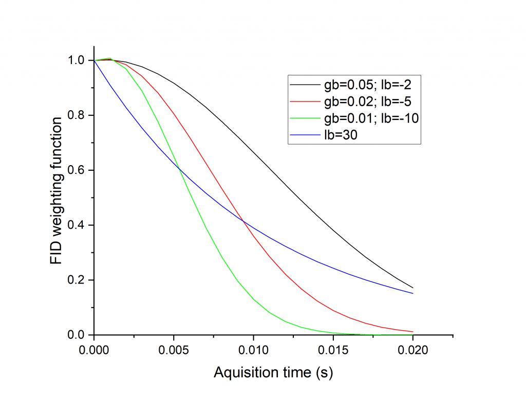
The figure below shows the weighting function for a number of line broadening choices (for an acquisition time of 20 ms). You can see that the several Gaussian curves retain the beginning part of the FID better than exponential (blue curve).

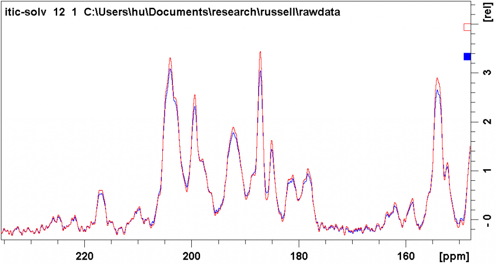
The figure below shows the different effect of the two types of line broadening. The blue spectrum was processed with exponential line broadening, with lb = 30 Hz. The red spectrum was processed with Gaussian line broadening, with gb = 0.03 and lb = -3. You can see that both ways suppress noise to a similar degree, while the latter way results in less peak overlap (deeper valleys between peaks).