There is a much easier way to run NOESY than the old 1D NOE-difference and the 2D NOESY:

1. first, run a proton spectrum.
2. with the spectrum on screen, click Acquire, then click Options, then click Setup Selective 1D Experiments.
3. Follow the menu and its prompts; select the peak(s) that you want to probe.
4. Click Create Datasets, select Selective gradient NOESY:

5. the computer will ask you to confirm some experimental parameters. The default choices are usually good. For each of the peak area that you select, one experiment will be run, and it will be stored under the same sample name, in incremental experiment numbers.

Following is a proton spectrum (blue) of pamoic acid and two selective NOESY spectra. Each took less than 1 minute. You can immediately see which proton is spatially close to the targeted protons (the large negative peak).

Related link: How to minimize DOSY artifacts due to convection

1. In Topspin, go to Help -> Manuals, find “DOSY” handout. Read and understand the principle.

2. rsh shim.best; lock; topshim; collect a standard proton spectrum (atma; rga; zg); calibrate 90deg pulse.

3. In edc window, click Experiment. in “…/user” directory, choose experiment DIFFUSION1D. check getprosol box.

3a. After you have created the new file, update p1 with the value that you have just obtained in step 2.

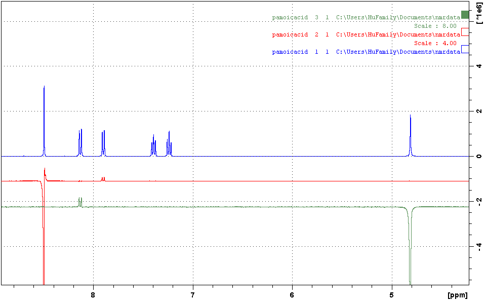
4. Run a spectrum. This one is with gpz6 = 2 (default; means 2% of the gradient amp power is used).

5. Create a new experiment by edc and choose “Use current parameters“. If your getprosol box is automatically checked, please uncheck it (if you don’t do this, the new file will use the spectrometer default pulsing parameters instead of the ones that you have just calibrated). Don’t do rga. type gpz6 and enter 95 (give the gradient amp 95% of the power). run the experiment.

5a. If the tall and sharp peaks have negative spikes on their sides that cannot be fixed by phase correction, type loopadj, then rerun the experiments.

6. compare the two spectra with 2% and 95% gradient powers (you can use the Multiple Display function to do this). You usually need the latter to be about or less than 1% of the former to obtain an accurate diffusion coefficient (D). You will need to adjust d20 to achieve this. d20 could range from 0.02 s to 0.5 s. The longer the d20, the deeper is the decay. Every time you change d20, you need to rerun both experiments.

6a. If your target peak cannot achieve this much decay within this window of d20, you will need to adjust another parameter, p30. p30 is the length of the gradient pulse and you will need to be extra careful as an erroneous value could burn the gradient amplifier and damage the probe, resulting in several thousand dollars of repair cost. The default p30 is 1000 us (microseconds). The maximum p30 that you can use is 2500 us. The default unit of p30 is us, so if you input 2500, the instrument will interpret it as 2500 us.

7. Once an optimal d20 (and optionally p30) is decided, create another new file by choosing DIFFUSION2D. change d20, p30, and p1 to the values that you have determined. Enter a suitable NS (should be multiple of 16). enter command dosy 2 95 16 q y y. This is a macro that will run a 2D DOSY expt. Meaning of the parameters: 2: beginning gradient amplitude = 2%; 95: ending gradient amplitude = 95%; 16: number of 1d slices = 16; q: increment is square rooted (alternatively, you could do l for linear increment); the first y: begin acquisition; the second y: do a rga before the run. For more details, please read the Bruker brochure mentioned in step 1. Note: if your target peak is overlapping with a large solvent peak, you could set the beginning gradient amplitude to be higher than 2%, say, e.g., 10%. This will greatly suppress the solvent peak intensity for your first data point and thus improve the quality of this point.

8. When done, click ProcPars tab and change SI of F1 column to 32. In command line, type xf2 to Fourier transform (only in the 2nd dimension). Correct phase. Only phase-correct rows. Then correct baseline.

9. type setdiffparm. This sends the experimental parameters that you used to Dynamics Center for data fitting.

10. on main menu, click Analysis -> T1/T2 module -> Dynamics Center. Or just type dync. Follow the flow in the new window. Instruction on using Dynamics Center can be found here.

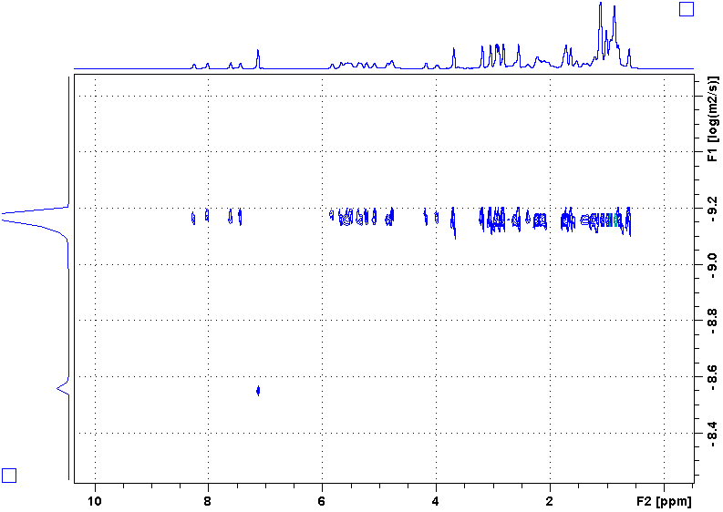
Following is a DOSY spectrum of cyclosoprin-A in benzene-d6. Most peaks are in the upper row while there is only one peak in the lower row. Why?

Following is a 31P kinetics spectrum run on the 500, collected by Zak Page. Over the course of the reaction, the decrease of the reactant peaks at 28 ppm, the increase of the product peaks at 1 ppm, and the first increase, then decrease of the intermediate signal at 27 ppm can be clearly seen. The time scale of the F1 dimension is erroneous (a software glitch).

(Unfortunately, this experiment cannot be run on the 500 cryoprobe)

Comparing 19F spectra with and without 1H decoupling can probe the interaction between 19F and neighboring 1H.

Here is a comparison. Sample: (CF3)2COOH in 90/10 H2O/D2O. Note that the 19F-1H J coupling is ca. 8 Hz even though they are four bonds away. (run on the old DPX300. Now gone)

Cr(acac)3 works every well in organic solvents for speeding up T1 relaxation, but does not dissolve in water.  A good choice of water soluble T1 relaxation agent is GdCl3.  Recommended concentration is 0.1-0.3 mg/ml.

This method is also good for water-swellable solid samples – prepare a GdCl3 solution and swell your polymer sample in the solution, and you have finally found a solution to your challenging signal intensity problem!

1. Set up your solvent suppression standard file (you only need to do this once).

(a) create a blank file from any template. Name it something like “standard-watersup”

(b) type rpar, select “…/user” directory, then select “ZGPR1”. Click OK on the window that subsequently pops up.

(c) type getprosol to complete setup. (you could also complete steps (b) and (c) by checking appropriate boxes in the edc window).

2. Find the frequency of the solvent (most frequently water) peak. You will need to do this every time you run a solvent suppression experiment. Water suppression only works when the frequency of your pulses is exactly on the water peak.

(a) run a regular proton spectrum;

(b) zoom in your solvent peak on the screen;

(c) click this button (set RF by cursor):

(d) left click on solvent peak top, and the following window will pop up. Write down the frequency shown in the pink blank:

(e) click Cancel.

3. Run experiment.

(a) create a new file from your standard water suppression file;

(b) type o1 (o stands for offset), enter the value you recorded in Step 2.

(c) run your expt like you do any other NMR expt (rga, zg).

(d) use manual phase correction as apk often has a hard time dealing with the somewhat distorted water peak. phase it such that your solute peaks are correctly phased, which might mean that the solvent peak has to be left out of phase. This will be addressed in the next step.

4. Optimization

(a) display a spectrum range of ca. 1 ppm wide with the solvent peak roughly in the middle. Type dpl1. This defines the spectral range that will be displayed during parameter optimization.

(b) type paropt (which stands for parameter optimization). You will be asked several questions: (1) parameter to optimize. enter o1. (2) beginning value. e.g. if the o1 determined in the last step was 2350Hz, enter 2345. (3) increment. enter 1. (4) number of experiments. enter 11. This will run 11 experiments with o1 ranging from 2345 to 2355.

(c) tighten the paropt step size and find the best solvent suppression. When the suppression is best, the out-of-phase water peak problem will be minimized. You might have to use 0.01 Hz step size to find the best suppression.

Molecule: 2-alkyl-benzimidazole

Red spectrum: regular 13C

Blue spectrum: 13C with Cr(acac)3 using the setup procedure described in this blog entry.

Both were run at ca. -24degC. Both took ca. 45 min.

Cr(acac)3 is especially powerful in speeding up the T1 relaxation of unprotonated 13C.

Sample: ca. 3 wt% regio-random P3HT in CDCl3.

Red spectrum is regular 13C. experiment time = 28 min.

Blue spectrum is DEPT135. experiment time =18 min. S/N is about 3 times better, with about 1/2 of experiment time compared to regular 13C. Also clarifies assignment of protonated vs non-protonated carbon peaks.

It is straightforward to setup and run the DEPT experiment. Refer to the “Training Materials” section of this blog to find out.

NOE effect is a powerful tool to probe spatial relationship between atoms in a molecule.  2D NOESY is a relative easy experiment to set up.  However, samples with small concentration have challenging signal sensitivity for 2D NOESY.  In such cases, 1D NOE Difference Spectroscopy is an excellent alternative.

1. For best NOE, sample need to be degassed to remove dissolved oxygen gas which is paramagnetic and will compete with NOE.  Nonpolar solvents are particularly capable of dissolving a large amount of oxygen gas, which could make NOE vanish.  Several cycles of freeze-pump-thaw of an uncapped NMR tube would remove most of the dissolved oxygen gas.
2. Run a standard proton spectrum
3. Take note of the chemical shift values of (A)the peak that you want to irradiate and (B) an irrelevant peak (eg. Solvent or TMS)
4. With this proton file on screen, create a new file by edc. Then type rpar and choose NOEDIFF. Then input the o2p value of the targeted proton peak.  Collect a spectrum (A).  Phase correct it.
5. Use spectrum A to create another 1D NOE new file and input the o2p value of the irrelevant peak.  Do not do rga – you need to use the same rg as in A.  Collect a spectrum (B).
6. Integrate spectrum B and save the integrals.
7. Load spectrum A.  In Multiple Display mode, load spectrum B and subtract the two spectra. Click “Save”, and you will be asked a “PROCNO”. Type 2. This will save the difference to processing number 2 within the same experiment (assume it is exp # 1).
8. Read in the difference file by typing re 1 2. The difference spectrum should have the irradiated peak negative and the NOE-enhanced peaks positive.
9. Integrate the difference spectra.  Right click on the NOE-enhanced peak integration curve and select “Use last scale for calibration”.  The ratio between this area and the area obtained in Step 6 is the NOE enhancement ratio.

First, you will need to create a standard file.  Create an empty file by typing edc.  Then type rpar, which brings up a big window.  Look for the nuclei of interest, eg., P31, Si29, B11, etc., and click on the choice, then click OK.  Then you must type getprosol to complete the standard file setup.

Once you have the standard file, the rest is similar to running a 1H or 13C experiment.  On 400, you will need to run atma.

Some nuclei have several options in the rpar window.  For example, P31CPD is P31 with proton decoupling, while P31 is without the decoupling.  You can run both and compare the spectra and look for the difference.

F19 only works on DPX300 (B622 Conte).  You can only select F19 (not F19CPD) in rpar window.  31P and 13C work on both DPX300 and Avance400 (LGRT room 075).  All other nuclei can only be done on Avance400.