Professor Vicic of Lehigh University created a database for 19F NMR.
Author Archives: Weiguo Hu
Are Polymer NMR Peaks Always Broad?
Solution NMR peak widths are mostly determined by two factors, homogeneous broadening and inhomogeneous broadening. Homogeneous broadening is governed by T2 relaxation, which is driven by the dynamics of the molecular segments. Small molecules rotate very fast in solution (>> 109 s-1), resulting in long T2 (~ seconds) and thus very sharp peaks (intrinsic peak width usually < 0.5 Hz). For polymers, there are different situations. For hydrocarbon polymers, each bond of the backbone rotates independent of the bonds that are more than 4-5 bonds away, and such rotations are almost as fast as those of small molecules. Therefore, NMR peaks of hydrocarbon polymers are almost as sharp as those of small molecules, and the peak widths are largely independent of molecular weight. For polymers that have strong interactions with solvents, the bond rotations might not be that free, resulting in shorter T2 and thus broader peak widths. You could think of the former case as a snake freely swirling in water while the latter case as a stiff coil of steel wire.
Inhomogeneous broadening is governed by the heterogeneity of chemical structure of the molecule. For example, a purely isotactic polymer has a uniform chemical structure throughout the backbone, while an atactic polymer has many different local structures (mmr, mrm, mrr, etc.). Therefore, an isotactic polystyrene has very sharp NMR peaks, while an atactic polystyrene has quite broad NMR peaks. The difference here is not homogeneous broadening due to T2 relaxation, but due to inhomogeneous broadening due to tacticity. In other words, the broad peaks on polystyrene NMR spectra are in fact many sharp peaks right next to each other.
In summary, polymer peaks are not always broad, and shimming is generally recommended for polymer samples. In fact, the extent of the peak broadening tells you a lot about the behavior of these molecules and their interaction with their surrounding environment.
Gaussian Line Broadening
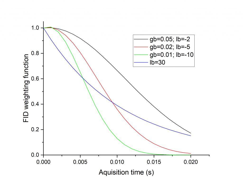
There are many choices of line broadening functions. The most popular one is exponential line broadening, in which each time-domain data point in the FID is given an exponentially decaying weight before Fourier Transformation. The drawback of exponential line broadening is that it suppresses the beginning part of FID too quickly, which results in long tails on the feet of tall peaks on the spectrum. If you want to cut those tails and reduce peak overlap yet still suppress a lot of noise, you could try Gaussian line broadening, in which you need to define two parameters: gb and lb. gb is between 0 and 1, while lb should be a negative number.
Gaussian line broadening is often used in the processing of solid-state NMR spectra, where peak overlapping issues are often severe. However, if you find peak overlapping is an issue in processing solution NMR spectrum (for example, if you want to resolve a small peak on the feet of a big peak), consider giving it a try. If you choose to do Gaussian instead of exponential line broadening, you will need to first define gb and lb, then type gfp instead of efp.
The Gaussian line broadening parameter pairs that I usually use are (from strongest to weakest):
gb / lb
0.01 / -10
0.015 / -8
0.02 / -5
0.03 / -3
0.05 / -2
0.1 / -1
The figure below shows the weighting function for a number of line broadening choices (for an acquisition time of 20 ms). You can see that the several Gaussian curves retain the beginning part of the FID better than exponential (blue curve).
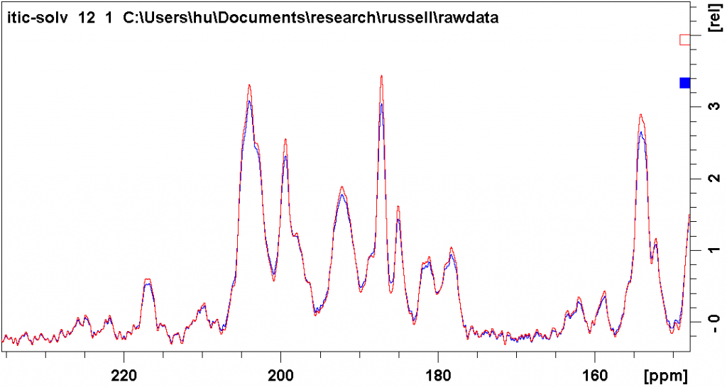
The figure below shows the different effect of the two types of line broadening. The blue spectrum was processed with exponential line broadening, with lb = 30 Hz. The red spectrum was processed with Gaussian line broadening, with gb = 0.03 and lb = -3. You can see that both ways suppress noise to a similar degree, while the latter way results in less peak overlap (deeper valleys between peaks).
Polymer Molecular Weight Prediction Models for DOSY NMR
This report includes prediction models for PS, PEO, and PMMA, as well as discussions on the models’ application and limitations, and practices for producing high-quality DOSY NMR data. Access is currently limited to the University of Massachusetts Amherst campus community only.
Advanced Baseline Correction
In some cases the automatic baseline correction command abs does not generate a desired baseline. This often happens when some of your peaks are broad and the correction algorithm has a hard time decide whether some data points in a certain spectral area is signal or baseline. In such cases, you can try an advanced baseline correction method: bas. Upon giving the command bas, you are offered a number of choices. I use the first and the third choices most often.
Choice 1, manual baseline correction. The correction is done by manual fitting of the baseline by a fifth order polynomial: y = A + Bx + Cx2 + Dx3 +Ex4 + Fx5. First, you display the range of the spectrum that you want to correct (note: you can baseline correct a small range of the spectrum instead of the entire spectrum). Second, You drag each of the five buttons A, B, C, D, and E to adjust the red baseline until it passes through the spectral baseline. I found that adjusting A, B, and C is often good enough. Finally, you click the “Return, Save regions” button, which will perform the correction. This option is very useful if you want to integrate a small peak riding on the shoulder of a big peak.
Choice 3, “Auto Correct Spectral Range…. only”. You need to decide two factors for this correction method: (1) a chemical shift range of spectrum for which you want baseline correction (ABSF1 and ABSF2). Since it is often difficult to perfectly correct baseline across the entire spectrum, only correcting a smaller range often produces better result. For this, you will need to properly choose the left and right limit of the range that you want the baseline correction be done. Choose the limits such that there are at least 0.5 ppm wide of signal-free regions at both ends of your spectral window. This will help the correction algorithm to recognize the baseline. (2) Shape of the polynomial (ABSG). I often find that lower orders of polynomial (0, which means that I only correct a constant offset A; 1, which means I only use the shape A + Bx; or 2, which means I only use the shape A + Bx + Cx2) do a better job than the ones that use all five orders, which often overdo the job.
Multi-Component Fitting of a Curve
We often encounter decay behaviors that cannot be accurately described by a single exponential curve, e.g. in T1 relaxation curves and in diffusion NMR data. In such cases, multi-component fitting of the curves could be attempted.
See the following diffusion NMR data:
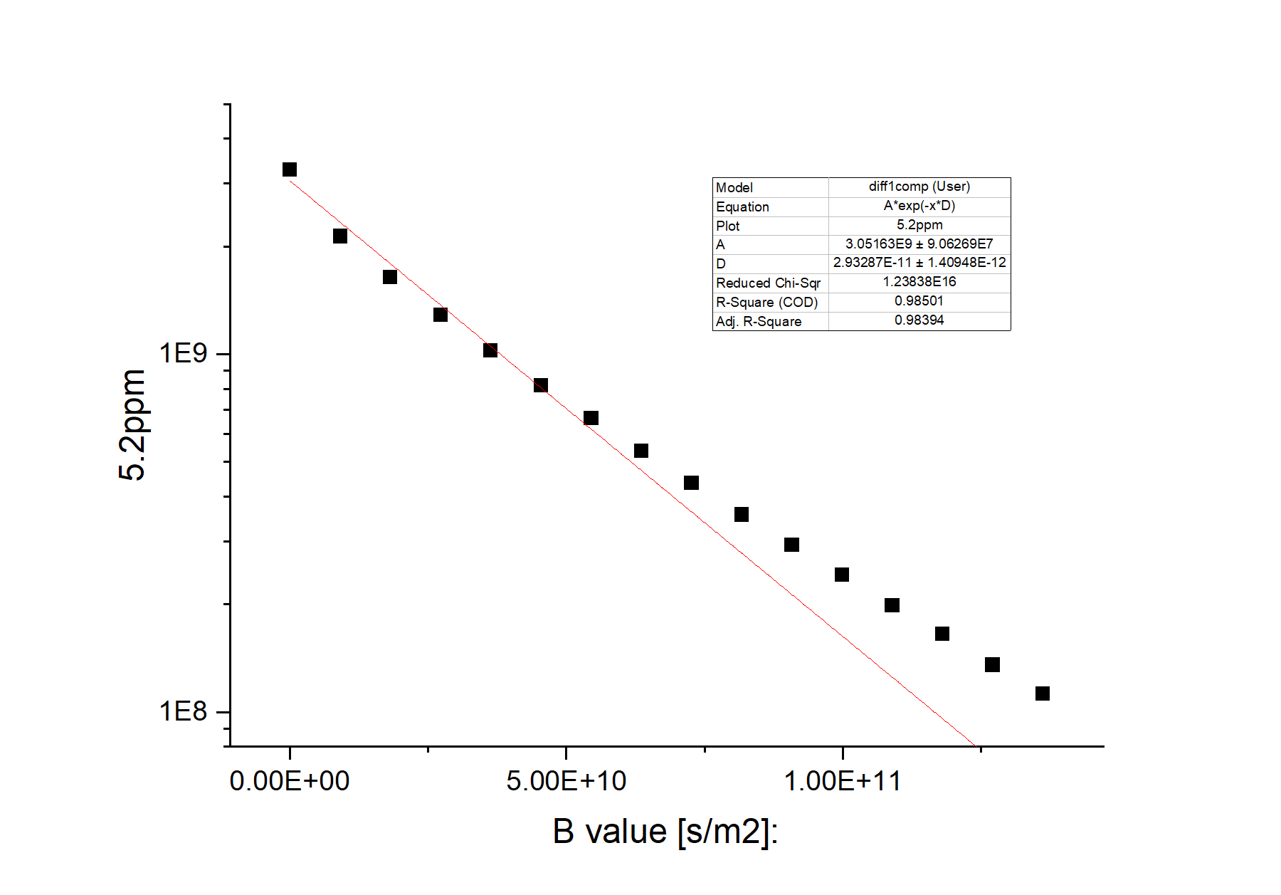
There is clearly a systematic deviation between the experiment data (black dots) and the single-exponential fit (red straight line). The resulting diffusion coefficient (D) has a relative error bar of ca. 5%. Upon close visual examination, we can notice that the experimental data decays faster in the beginning and decays slower toward the end. So a two-component fit might produce better results.
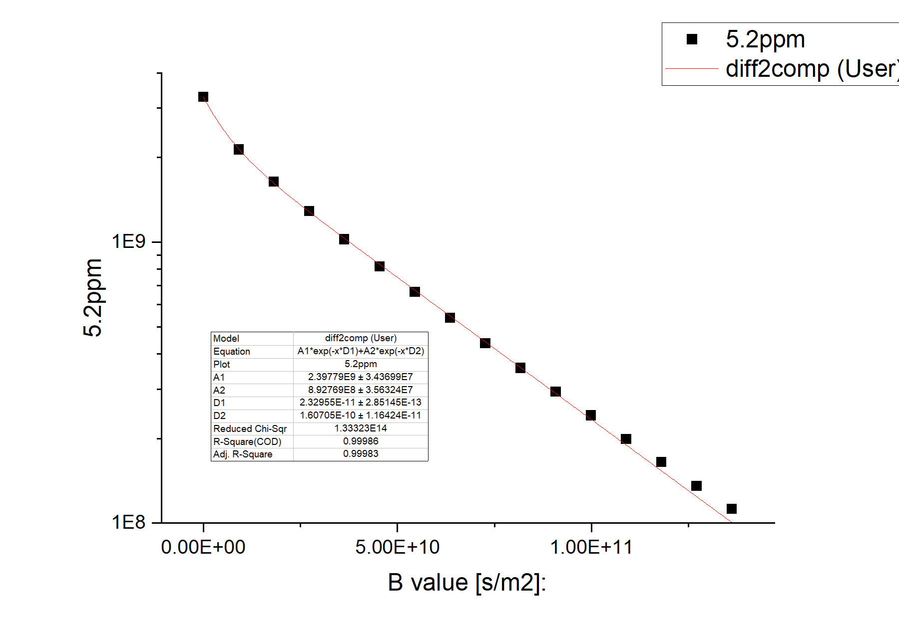
The equation of the two-component fit function can be seen in the inset of the figure above. The fitting quality is clearly much better. The reduced chi-square is two orders of magnitude smaller. A1 and A2 are the amplitudes of the two components, while D1 and D2 are their diffusion coefficients. Comparison of the two figures shows that a two-component system is a much better representation of the sample.
Hydrogen Bonding Probed by 15N NMR
The nitrogen site of pyridine is a hydrogen bond acceptor. In the presence of a hydrogen bond donor, its 15N peak shifted upfield by more than 1 ppm. See picture below (blue: pyridine; red: pyridine + H donor). This is one way of probing the presence of hydrogen bond in solution.
a
How to Compare Integrations for Different Data Files
You can compare the signal integration of different data files. They will need to be acquired with the same receiver gain (rg). To ensure this, before you run your first sample, run rga, then type rg to record the receiver gain that has been determined. When you run your other samples, instead of running rga, you type rg and input the receiver gain that you wrote down for your first sample. This will ensure all the spectra that you want to compare signal areas against have been run with the same receiver gain.
It is possible to use different ns for different samples, but you will need to remember that signal area is proportional to number of scans and thus properly normalize your peak areas against ns.
When comparing peak areas, after integrating your first sample, save the integration results and return to main menu. Then do your second sample. Before you exit the integration mode, right click on the integration screen and select “Use lastscale for calibration” (see picture below). The peak areas will be rescaled such that the peak areas for your current sample will be quantitatively comparable to your last one.

Course Syllabus for PSE797DD
How to run a 2H experiment
If you want to investigate the structure and behaviors of deuterium in your molecules, 2H NMR is a good method. The chemical shift of 2H is very similar to that of 1H as both nuclei experience the same electron environments. The resolution is also often as good as that for 1H.
Follow these steps:
- Type edc. In Experiment, choose H2. Check getprosol box. Create a new file for 2H experiment.
- Type rsh shims.best
- If your sample is dissolved in a deuterated solvent, do the regular lock and shim
- If your sample is not in a deuterated solvent, type ii. This will stop the locking mechanism from interfering with your 2H experiment. Often, your spectral resolution is already good enough so that you do not need to further shim. If you need high resolution, you will need to manually shim on the FID: Type gs (similar to zg but without accumulating data, used for real time adjustment of various parameters), then adjust z and z2 in bsmsdisp window to make the FID as long and thick as possible.
- Type atma
- Type rga
- Run your experiment. Adjust d1, ns, and lb as needed.